Cross-Validation: Concept and Example in R

Cross-validation, sometimes called rotation estimation, is a model validation technique for assessing how the results of a statistical analysis will generalize to an independent data set. It is mainly used in settings where the goal is prediction, and one wants to estimate how accurately a predictive model will perform in practice.

In Machine Learning, Cross-validation is a resampling method used for model evaluation to avoid testing a model on the same dataset on which it was trained. This is a common mistake, especially that a separate testing dataset is not always available. However, this usually leads to inaccurate performance measures (as the model will have an almost perfect score since it is being tested on the same data it was trained on). To avoid this kind of mistakes, cross validation is usually preferred.

The concept of cross-validation is actually simple: Instead of using the whole dataset to train and then test on same data, we could randomly divide our data into training and testing datasets. The aim in cross-validation is to ensure that every example from the original dataset has the same chance of appearing in the training and testing set.

There are several types of cross-validation methods (Monte Carlo cross validation, LOOCV – Leave-one-out cross validation, the holdout method, k-fold cross validation). Here, emphasis would be placed only on K-Fold cross validation method.
K-Fold  basically consists of the below steps:

1. Randomly split your entire dataset into k”folds”.
2. For each k folds in your dataset, build your model on k – 1 folds of the data set. Then, test the model to check the effectiveness for kth fold.
3. Record the error you see on each of the predictions.
4. Repeat this until each of the k folds has served as the test set.
5. The average of your k recorded errors is called the cross-validation error and will serve as your performance metric for the model.

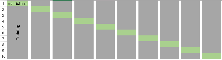
Below is the visualization of how does a k-fold validation work for k=10. copies from Analyics Vidhya

Building a Model

Firstly, we’ll load in our data:

train <- read.csv(url("http://s3.amazonaws.com/assets.datacamp.com/course/Kaggle/train.csv"))

and do a quick screening:

str(train)
table(train$Survived)
prop.table(table(train$Survived))

We have 891 observations, with 549 (62%) people who died, and 342 (38%) people who survived.

Information on the variables in the Titantic dataset can be found here. For our model, we’ll use a decision-tree model with passenger class (“Pclass”), sex (“Sex”), age (“Age”), number of siblings or spouses aboard (“SibSp”), number of parents or children aboard (“Parch”), the passenger fare (“Fare”) and port of embarkation (C = Cherbourg; Q = Queenstown; S = Southampton) (“Embarked”).

library(rpart); library(caret)
model.single <- rpart(Survived ~ Pclass + Sex + Age + SibSp + Parch + Fare + Embarked, 
                      data = train, method = "class")
predict.single <- predict(object = model.single, newdata = train, type = "class")

library(RGtk2); library(cairoDevice); library(rattle); library(rpart.plot); library(RColorBrewer)
fancyRpartPlot(model.single)

Now let us examine the model performance on trained data.

confusionMatrix(predict.single, train$Survived)

## Confusion Matrix and Statistics
## 
##           Reference
## Prediction   0   1
##          0 521 115
##          1  28 227
##                                          
##                Accuracy : 0.8395         
##                  95% CI : (0.8137, 0.863)
##     No Information Rate : 0.6162         
##     P-Value [Acc > NIR] : < 2e-16        
##                                          
##                   Kappa : 0.6436         
##  Mcnemar's Test P-Value : 6.4e-13        
##                                          
##             Sensitivity : 0.9490         
##             Specificity : 0.6637         
##          Pos Pred Value : 0.8192         
##          Neg Pred Value : 0.8902         
##              Prevalence : 0.6162         
##          Detection Rate : 0.5847         
##    Detection Prevalence : 0.7138         
##       Balanced Accuracy : 0.8064         
##                                          
##        'Positive' Class : 0          

The accuracy of the model is 0.839 when applied to trained data. However, this is likely to be an overestimate/overfitting. The best bet to get a more accurate and unbiased model is to apply the modul on new data also called test data.

The usual way to do this is to split the dataset into a training set and a testing set, build the model on the training set, and apply it to the testing set to get the accuracy of the model on new data. Cross-validation is kind of the same idea as creating single training and testing sets; however, because a single training and testing set would yield unstable estimates due to their limited number of observations, you create several testing and training sets using different parts of the data and average their estimates of model fit.

K-fold cross-validation

In k-fold cross-validation, we create the testing and training sets by splitting the data into k equally sized subsets. We then treat a single subsample as the testing set, and the remaining data as the training set. We then run and test models on all k datasets, and average the estimates. Let’s try it out with 5 folds:

k.folds <- function(k) {
    folds <- createFolds(train$Survived, k = k, list = TRUE, returnTrain = TRUE)
    for (i in 1:k) {
        model.train <- rpart(Survived ~ Pclass + Sex + Age + SibSp + Parch + Fare + Embarked, 
                       data = train[folds[[i]],], method = "class")
        predictions <- predict(object = model.train, newdata = train[-folds[[i]],], type = "class")
        accuracies.data <- c(accuracies.data, 
                           confusionMatrix(predictions, train[-folds[[i]], ]$Survived)$overall[[1]])
    }
    accuracies.data
}

set.seed(007)
accuracies.data <- c()
accuracies.data <- k.folds(5)
accuracies.data

## [1] 0.8033708 0.7696629 0.7808989 0.8435754 0.8258427

mean.accuracies <- mean(accuracies.data)

As you can see above, this function produces a vector containing the accuracy scores for each of the 5 cross-validations. If we take the mean and standard deviation of this vector, we get an estimate of our out-of-sample accuracy. In this case, this is estimated to be 0.81, which is quite a bit lower than our in-sample accuracy estimate.

Finally, you can apply the model to a test set. Hope you are able to get a meaningful insight into cross valisation and how it is an essential tool for Data-scientist. for more information you can visit http://t-redactyl.io/blog/2015/10/using-k-fold-cross-validation-to-estimate-out-of-sample-accuracy.html